Associations Between Tree Species Occurrence and Neighborhood Income in the Urban United States
Eli Robinson
2023-09-12
Abstract
This study aimed to understand if there was a connection between tree species and income levels in ten different cities in the US, using data from the Urban Forest Inventory and Analysis (FIA) dataset and demographic information from the 2020 US Census Bureau American Community Survey at the census block group level. The Urban FIA dataset provides detailed information on urban trees, including diameter, height, condition, biomass, and species. The study used spatial analysis to investigate associations between tree species and the average household income of the surrounding neighborhood. The results showed that tree species occurrence varied with local income, with some species appearing more frequently in high-income areas, while others were more common in low-income areas. The ecosystem services and disservices provided by trees vary among species, implying associations between neighborhood income and both positive and negative human-plant interactions. These results provide a path towards understanding tree-related inequity in American cities and future research on this topic could help inform policy and tree management decisions that aim to reduce ecological inequity.
Introduction
Trees have major effects on cities by reducing urban heat island effect, mitigate air pollution, improve drainage, and provide health benefits to humans (Speak, 2018; Wolf, 2020). Every tree, however, provides different services. Each tree species provides a different value of ecosystem service to the environment it is in, and differences among tee species are often overlooked when urban tree studies are performed. For example, certain woods and trees provide different abilities to filter air pollution (Chen 2017), have different cooling potentials (Rahman, 2020), and have different pollen exposure risks (Sousa-Silva, 2021). It is important to understand the spatial distribution of these urban trees across urban areas and across different socioeconomic groups in order to understand if there are differences in tree composition as a function of neighborhood demography (e.g., income). Differences in tree composition as a function of income could result in inequity in the ecosystem services and disservices provided by urban trees. Understanding any such inequity in tree composition is the first step towards potential policy and management goals of reducing inequity in the services provided by trees.
Previous research has been done in this area of study including studies that measured canopy cover related to urban heat (McDonald, 2021). This study measured the differences between overall tree cover and urban heat and found that with less tree cover there is more heat. McDonald et al. found that tree cover was also correlated with socioeconomic factors. Another study compared green spaces to socioeconomic conditions (Li, 2015) and found that areas of lower socioeconomic status had fewer green spaces. These studies and many similar studies use imagery to quantify tree cover (e.g., Landsat imagery or Google Street View). These methods are good for quantifying green spaces or tree cover but are unable to provide key information on tree species composition.
Anecdotal evidence suggests that tree species composition varies across income levels within cities, however this has not been systematically assessed across cities. If so, this could have implications for the ecosystem services and disservices provided by trees, which could have policy and management implications. A new program, the Urban Forest Inventory and Analysis (UFIA) is measuring trees in urban areas and provides the first systematic and uniform dataset that could be used to compare tree identity and neighborhood demography in cities across the United States. Here, I combine UFIA and data from the US Census Bureau to quantify associations between tree species and income levels in 10 cities in the United States.
Methods
Two data sets that were used for this study: the first is census block group information from 2020 US Census Bureau American Community Survey (Manson, 2022) focusing on average household income. Census block group is the finest resolution data that has the average household income so that it was used for this study. The census variable used for this study is AMRE8001 which is the median household income in the past 12 months (in 2020 inflation-adjusted dollars).
The UFIA dataset (Edgar, 2021) is a relatively new dataset of urban trees. This dataset differs from the remote sensing data that several studies have used to compare to socioeconomic data because the UFIA data is collected by surveyors on the ground. This allows for additional information to be collected including diameter of a tree, height, calculated biomass, condition of tree, and tree species. This is the first federal program which conducts representative studies and data collection of trees in urban areas. This data set contains a set of tree and plot data that contains information about urban trees including location, species, condition, and much more with both measured and calculated values. This dataset has information for 10 cities (Austin, TX; Chicago, IL; Houston, TX; Kansas City, MO; Portland, OR; San Antonio, TX; San Diego, CA; Springfield, MO; St. Louis, MO; Washington DC) across the US which will be the areas of focus for this study. Additional UFIA censuses are currently ongoing in 34 other cities.
The goal of the project was to investigate associations between tree species occurrence and neighborhood income. In order to do this the UFIA data has trees within plots, which have location values associated with them. In order to conduct spatial analysis on tree information it is necessary to combine this information at some point. First, however, I must find the average household income associated with each plot. The divulged coordinates of UFIA plots are only accurate to within 1 km. To account for this, I buffered each plot by 1 km. I intersected the resulting buffer with the census block groups and averaged the income, weighted by the census block group area that was within the buffer. Then I dissolved by plot. This results in the area of the buffered plot with the information of the weighted local census information. Census information for the buffered area was then merged with the UFIA tree data. This gives each tree both a geometry of their plot location and the average household income of the nearby block groups.
The result is a dataset of trees which has species name from the original dataset and local income value from the spatial analysis. In order to display results, I plotted the 5 most common tree species in a city by the mean local income found via the spatial analysis. This will give an understanding of some of the common tree species in each city and how they relate to the local income. I also mapped the plots across the city colored by species in order to better understand the spatial context of each city. To test whether tree occurrence varied among income levels I used an ANOVA and then a Tukey’s HSD (honestly significant difference) test.
This analysis was done in Python 3 using the Pandas and Geopandas libraries for spatial analysis and Seaborn for plotting and visualization, SciPy for statistics, NumPy for arithmetic, as well as other small libraries for easy access. The codebook can be found here on the website (https://eli-robinson.github.io/UrbanFIAAnalysis/FIASpecies.html) and also on the public GitHub repository (https://github.com/Eli-Robinson/UrbanFIAAnalysis) which can be cloned for further research.
Results
In order to display results we plotted the 5 most common tree species in a city by the mean local income found via the spatial analysis. This will give an understanding of some of the common tree species in each city and how they relate to the local income.
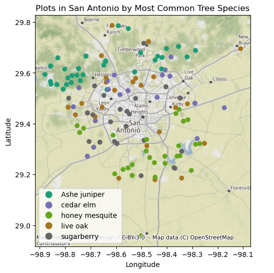 Fig. 1 shows a map of San Antonio with the plots where the five most
common species are. This map shows many Ashe juniper (Juniperus
ashei) trees in the northern areas of the city and many honey
mesquite trees (Prosopis glandulosa) on the southern block of
the city with sugarberry, (Celtis laevigata) and cedar elm
(Ulmus crassifolia) more in the center and downtown areas and
live oak (Quercus virginiana) seems to have been spread around
the entire city. This map and others of different cities can help to
provide additional context for the following results.
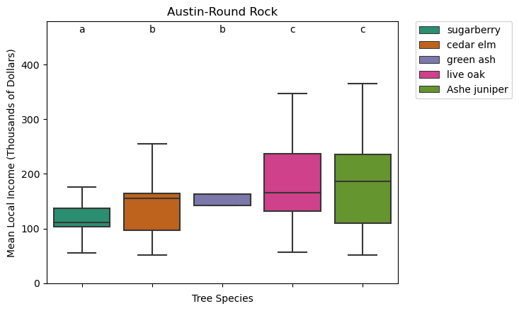
Figure 2: Association between tree species occurrence and neighborhood income in Austin, Texas, filtered by the top five most commonly occurring species. The line in the box shows median value, the box max and minimum are one quartile, and the whiskers show the maximum and minimum values dismissing outliers. Species that do not have a shared letter above them are statistically significant in terms of mean income.
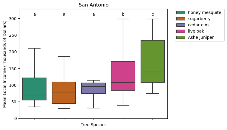
Figure 3: Association between tree species occurrence and neighborhood income in San Antonio, Texas, filtered by the top five most commonly occurring species. The line in the box shows median value, the box max and minimum are one quartile, and the whiskers show the maximum and minimum values dismissing outliers. Species that do not have a shared letter above them are statistically significant in terms of mean income.
These first two graphs of Austin, Texas (Fig. 2) and San Antonio, Texas (Fig. 3) are quite similar. Four of the five most common trees in the city are shared between the two, and each show similar results, with sugarberry on the low end, cedar elm towards the middle of the income and, ashe juniper and live oak towards the higher end of the average local income.
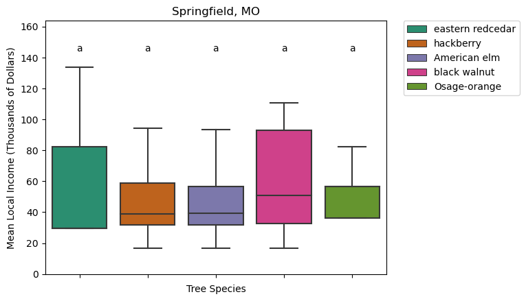
Figure 4: Association between tree species occurrence and neighborhood income in Springfield, Missouri, filtered by the top five most commonly occurring species. The line in the box shows median value, the box max and minimum are one quartile, and the whiskers show the maximum and minimum values dismissing outliers. Species that do not have a shared letter above them are statistically significant in terms of mean income.
When looking at the graph of Springfield, Missouri there are two things that stand out. The first is that all five of the common trees appear to be in the same income brackets. The other is that due to Springfield being a small city the mean local incomes of this city are much lower than some of the other cities that have been shown.
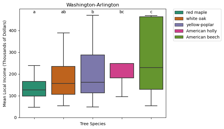
Figure 5: Association between tree species occurrence and neighborhood income in Washington D.C., filtered by the top five most commonly occurring species. The line in the box shows median value, the box max and minimum are one quartile, and the whiskers show the maximum and minimum values dismissing outliers. Species that do not have a shared letter above them are statistically significant in terms of mean income.
In Washington D.C. there is a difference between the common tree species with many American beech (Fagus Grandifolia) trees in wealthy areas and red maples (Acer rubrum) and white oak (Quercus alba) in the lower income areas. This graph shows a good spread between all the different species.
Discussion
The results of this study provide valuable insights into the relationship between income and tree species in urban areas. While similar studies have found that income is often a predictor of tree cover, with low-income neighborhoods having less tree cover than higher-income neighborhoods (McDonald, 2021; Li, 2015), the results presented here provide the nuance of tree species identity. In these urban areas, certain tree species tend to be more common in high-income areas, while other species are more commonly found in low-income areas.
All trees are not the same and different species of trees provide different ecosystem services such as trees with thicker leaves and denser foliage provide increased shading, and tree wood anatomy can provide increased transpiration. (Rahman, 2019). Different trees provide a wider range of benefits such as improved air quality, reduced energy use, and enhanced mental health. These differences in tree composition are therefore likely to affect the ecosystem services and disservices provided in rich vs poor neighborhoods; this work suggests that not all communities have equal access to these benefits. The findings in this study are particularly interesting because they shed light on potential inequities in urban forestry and urban tree management and highlight the need for a more equitable distribution of trees. Understanding the patterns of inequities is a crucial first step towards any eventual policy or management goals for improving environmental and social equity in urban areas.
One example of species that commonly appear in low-income areas, especially in Texas, is the sugarberry tree, Celtis laevigata (Willdenow). The sugarberry tree is a tree that is native to the southeast United States and is a short to medium sized tree that grows fast and can grow in a variety of soil types and conditions. This makes the sugarberry a very opportunistic tree as it can gain hold and grow in a variety of environments. The sugar berry tree being a small tree provides less tree cover, and environmental benefits than a larger and potentially more desirable tree. One such tree that appears in these Texas urban environments is the live oak tree. The live oak tree is a deep-rooted species which can help prevent erosion, and its larger size in width and increased leaf areas provide additional tree cover. This is just one example and there are similar species in high and low income areas in other cities as well.
Urban trees tend to shift more towards these invasive or opportunistic species when tree planting and management decrease (Nowak, 2012). One possible explanation for the patterns found here is that the tree planting and maintenance programs may be more common in higher-income neighborhoods which could create a disparity between neighborhoods of different socioeconomic status.
There are some limitations with the current methods. One of the limitations is data clustering, which is when there are many trees of the same species with the same value for mean local income. This occurs when there are many trees of the same species in one plot. Since the income is assigned by plot. All the trees are given the same mean local income which can cluster the data; future work should correct for this by including a random effect for plot within each city. Another limitation is the necessary one-kilometer buffering because the UFIA plot coordinates are intentionally jittered by up to 1 km. This buffering of the plots creates a larger range of incomes that are aggregated which in turn could create some inaccuracies of local income. These limitations are due to the nature of data collection and should be kept in mind but should not be detrimental to the study. In some cases, there are a few trees at a zero value for mean local income (e.g., in San Antonio). This is not due to being in an area where people have an income of zero but rather the trees are in areas where there are no people living. This could be business districts that are not zoned for living, parks and natural lands, or government buildings that have a relatively small block group size.
Future research could further explore the underlying causes of these patterns and identify potential solutions for improving equitable access to trees in urban areas. Additionally, continued monitoring and data collection efforts such as the UFIA program can help inform management and policy decisions. One example of future research that can be done based off this work is to fully map out the ecosystem service and disservice of each tree species. Creating a model based on literature such as Bolund, 2017 and other papers which can help to determine how valuable a tree is to the urban environment based on a variety of factors. This could assign the service and disservices provided by trees of each species and help to elucidate the connection between neighborhood demography, tree composition, and ecosystem services and disservices. Another piece of research that could be done is to use different information within the UFIA data. The UFIA data has many different variables which are all interesting and could each have individual studies on them. These studies could also make more sense across a broader scope of cities as tree species are generally most determined by environment rather than other factors such as tree height or condition, which are affected but may not be drastically different city by city.
In conclusion, species of trees in urban areas of the United States are associated with income, with some species corresponding to higher and some corresponding to lower income areas. This difference may result in different ecosystem services provided by trees, including pollen levels, amount of shade, and air filtration. Understanding where these differences lie is the first step towards ensuring each neighborhood has equal access and resources to the environmental services that all different tree species provide.
Works Cited
Andrew Speak, Francisco J. Escobedo, Alessio Russo, Stefan Zerbe, An ecosystem service-disservice ratio: Using composite indicators to assess the net benefits of urban trees, Ecological Indicators, Volume 95, Part 1, 2018, Pages 544-553, ISSN 1470-160X, https://doi.org/10.1016/j.ecolind.2018.07.048.
Edgar, Christopher B, et al. “Strategic National Urban Forest Inventory for the United States.” Journal of Forestry, vol. 119, no. 1, 2020, pp. 86–95, https://doi.org/10.1093/jofore/fvaa047.
McDonald RI, Biswas T, ddSachar C, Housman I, Boucher TM, Balk D, et al. (2021) The tree cover and temperature disparity in US urbanized areas: Quantifying the association with income across 5,723 communities. PLoS ONE 16(4): e0249715. https://doi.org/10.1371/journal.pone.0249715
Nowak, D. J. (2012). Contrasting natural regeneration and tree planting in fourteen North American cities. Urban Forestry & Urban Greening, 11(4), 374–382. https://doi.org/10.1016/j.ufug.2012.02.005
Per Bolund, Sven Hunhammar, Ecosystem services in urban areas, Ecological Economics, Volume 29, Issue 2, 1999, Pages 293-301, ISSN 0921-8009, https://doi.org/10.1016/S0921-8009(99)00013-0.
Rahman, M. A., Stratopoulos, L. M. F., Moser-Reischl, A., Zölch, T., Häberle, K. H., Rötzer, T., et al. (2020). Traits of trees for cooling urban heat islands: A meta-analysis. Building and Environment, 170, 106606. https://doi.org/10.1016/J.BUILDENV.2019.106606
Sousa-Silva, R., Smargiassi, A., Kneeshaw, D. et al. Strong variations in urban allergenicity riskscapes due to poor knowledge of tree pollen allergenic potential. Sci Rep 11, 10196 (2021). https://doi.org/10.1038/s41598-021-89353-7
Steven Manson, Jonathan Schroeder, David Van Riper, Tracy Kugler, and Steven Ruggles. IPUMS National Historical Geographic Information System: Version 17.0 [dataset]. Minneapolis, MN: IPUMS. 2022. http://doi.org/10.18128/D050.V17.0
Variation in tree species ability to capture and retain airborne fine particulate matter (PM2. 5) L Chen, C Liu, L Zhang, R Zou, Z Zhang - Scientific reports, 2017 - Springer https://link.springer.com/content/pdf/10.1038/s41598-017-03360-1.pdf
Wolf KL, Lam ST, McKeen JK, Richardson GRA, van den Bosch M, Bardekjian AC. Urban Trees and Human Health: A Scoping Review. International Journal of Environmental Research and Public Health. 2020; 17(12):4371. https://doi.org/10.3390/ijerph17124371
Xiaojiang Li, Chuanrong Zhang, Weidong Li, Yulia A. Kuzovkina, Daniel Weiner, Who lives in greener neighborhoods? The distribution of street greenery and its association with residents’ socioeconomic conditions in Hartford, Connecticut, USA, Urban Forestry & Urban Greening, Volume 14, Issue 4, 2015, Pages 751-759, ISSN 1618-8667, https://doi.org/10.1016/j.ufug.2015.07.006.